How to Use VLOOKUP in Google Sheets (with Examples)
VLOOKUP is the function that pulls a matching value from one table into another — the price for a product code, the email for a name, the region for a store. It looks intimidating, but it's really just four arguments. This guide walks through each one, then covers the real jobs people actually need it for: looking up from another sheet, across two separate files, on more than one condition, and fixing the #N/A error when a match won't come through.
VLOOKUP in Google Sheets uses the syntax =VLOOKUP(search_key, range, index, [is_sorted]). It finds search_key in the first column of range and returns the value from the column number you give as index. Always end with FALSE to force an exact match — e.g. =VLOOKUP(A2, Sheet2!A:C, 3, FALSE).
1. The syntax, one argument at a time
Every VLOOKUP has the same four parts:
=VLOOKUP(search_key, range, index, [is_sorted])| Argument | What it means |
|---|---|
search_key | The value you're looking for (e.g. a product code in A2). |
range | The table to search. VLOOKUP looks in its first column for the key. |
index | Which column of the range to return, counted from the left, starting at 1. |
is_sorted | Use FALSE for an exact match. (TRUE does an approximate match and needs a sorted column — rarely what you want.) |
Say you have products in columns A–C on a lookup table, and you want the price for the code in A2:
=VLOOKUP(A2, $A$8:$C$40, 3, FALSE)This finds the code from A2 in the first column of the table, then returns column 3 (price) from the matching row. The dollar signs lock the table range so you can drag the formula down without it shifting.
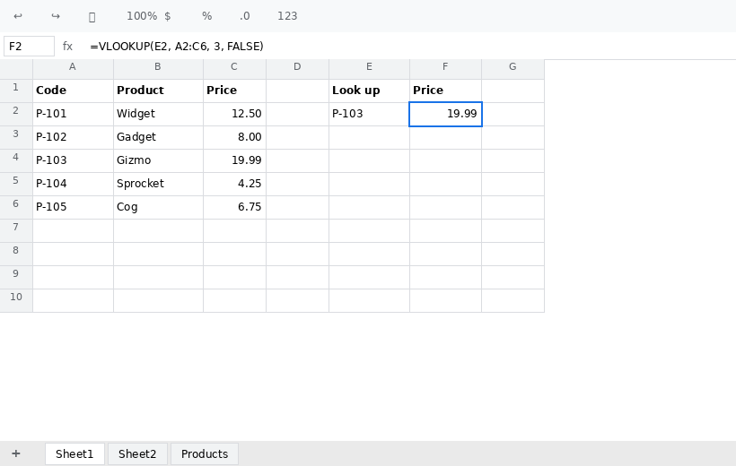
The #1 rule: VLOOKUP only searches the first column of your range and can only return columns to its right. If the value you want is to the left of your key, jump to INDEX/MATCH.
2. VLOOKUP from another sheet (tab)
How do I VLOOKUP from another sheet?
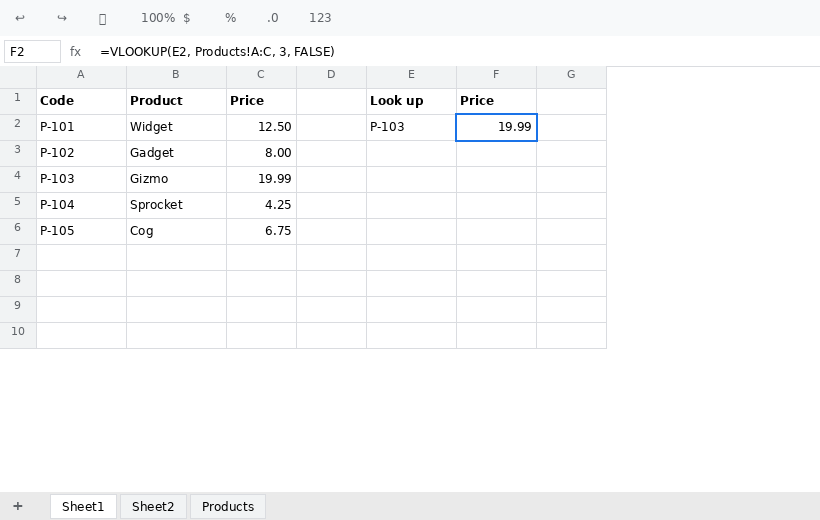
Put the tab name and an exclamation mark before the range: =VLOOKUP(A2, Sheet2!A:C, 3, FALSE). Everything else works exactly the same — only the range now points at the other tab.
This is the most common real-world use: your working sheet is on one tab, and the reference table (a price list, an employee roster) lives on another. Type the formula as usual, but when you select the range, click the other tab and highlight the columns there. Sheets writes the tab name in for you:
=VLOOKUP(A2, Products!A:C, 3, FALSE)If your tab name has a space in it, Sheets wraps it in single quotes automatically — ='Price List'!A:C. Using whole columns like A:C (instead of A2:C40) means new rows added to the reference tab are covered automatically.
3. VLOOKUP between two different files
Can VLOOKUP pull data from two separate spreadsheets?
Yes — wrap IMPORTRANGE inside VLOOKUP so the range comes from the other file: =VLOOKUP(A2, IMPORTRANGE("url","Sheet1!A:C"), 3, FALSE). The first time, click the cell and grant access when Sheets asks.
VLOOKUP can't reach another file on its own, but IMPORTRANGE can — it pulls a live range from a different spreadsheet, and VLOOKUP searches that. Use the other file's URL (or just its long ID) and the tab + range you need:
=VLOOKUP(A2, IMPORTRANGE(
   "https://docs.google.com/spreadsheets/d/FILE_ID_HERE",
"Products!A:C"), 3, FALSE)- The cell first shows
#REF!with a “Allow access” prompt — click it once to connect the two files. - After that it behaves like any other VLOOKUP and refreshes when the source changes.
Tip: IMPORTRANGE only needs the connection approved once per pair of files. If it breaks later, it's usually because the source tab was renamed or the sharing was removed.
4. VLOOKUP with multiple criteria
How do I match on two columns at once?
Standard VLOOKUP matches one column. To match on two (say region and product), join them into a single key with an array: =ARRAYFORMULA(VLOOKUP(A2&"|"&B2, {Sheet2!A:A&"|"&Sheet2!B:B, Sheet2!C:C}, 2, FALSE)).
The trick is to glue your two criteria together with a separator (|) so the pair becomes one lookup value, and build a matching virtual first column inside { }:
=ARRAYFORMULA(
   VLOOKUP(A2&"|"&B2,
   {Sheet2!A:A&"|"&Sheet2!B:B, Sheet2!C:C},
   2, FALSE))
Here the array {...} builds a two-column table on the fly: a first column that is region|product joined, and a second column with the value you want returned. The | separator prevents false matches (so “12” + “34” can't collide with “1” + “234”).
5. Partial matches with wildcards
How do I VLOOKUP a partial match?
Wrap your key in asterisks to match any cell that contains it: =VLOOKUP("*"&E2&"*", A:B, 2, FALSE). In VLOOKUP, * stands for any number of characters and ? for a single character — they only work when the last argument is FALSE.
This is how you look up “Apple” and still match a cell that reads “Apple Inc.” The asterisks tell VLOOKUP to accept anything before and after your text:
=VLOOKUP("*"&E2&"*", Products!A:B, 2, FALSE)   → contains E2
=VLOOKUP(E2&"*", Products!A:B, 2, FALSE)       → starts with E2
=VLOOKUP("*"&E2, Products!A:B, 2, FALSE)       → ends with E2
Matching a literal * or ?: put a tilde in front of it (~*) so Sheets treats it as a real character instead of a wildcard.
6. Case-sensitive lookups
Can I make VLOOKUP case-sensitive?
VLOOKUP ignores case by default — apple and APPLE match. To force case-sensitivity, swap in INDEX/MATCH with EXACT: =INDEX(B:B, MATCH(TRUE, EXACT(A:A, E2), 0)), which only matches an entry with the exact same capitalization.
VLOOKUP has no case-sensitive mode, so when SKU-a1 and SKU-A1 are different items, it will happily return the wrong one. EXACT compares two strings character-for-character including case, and MATCH(TRUE, …, 0) finds the first row where that's true:
=INDEX(B:B, MATCH(TRUE, EXACT(A:A, E2), 0))Return the value from column B on the row whose column-A entry exactly matches E2, capitalization and all.
7. Return several columns at once
How do I VLOOKUP and return multiple columns?
Pass an array of column numbers as the index and wrap it in ARRAYFORMULA: =ARRAYFORMULA(VLOOKUP(A2, Sheet2!A:D, {2,3,4}, FALSE)). One formula returns columns 2, 3 and 4, spilling into the cells to its right.
Instead of writing three separate VLOOKUPs to pull a name, email, and region for the same key, give the index a list in curly brackets:
=ARRAYFORMULA(VLOOKUP(A2, Contacts!A:D, {2,3,4}, FALSE))The result fills three adjacent cells in one go, and you can reorder the output by changing the list — {4,2,3} returns region, then name, then email.
8. When to use INDEX/MATCH instead
Can VLOOKUP look to the left?
No — VLOOKUP can only return columns to the right of the search column. When the value you need sits to the left, use INDEX and MATCH: =INDEX(A:A, MATCH(D2, C:C, 0)) finds D2 in column C and returns the same row from column A.
MATCH finds which row your value is on; INDEX returns the cell from that row in whatever column you point at — left or right. That makes the pair more flexible than VLOOKUP:
=INDEX(return_column, MATCH(search_key, lookup_column, 0))The 0 in MATCH means exact match (the equivalent of VLOOKUP's FALSE). INDEX/MATCH also doesn't break when you insert or delete columns in the middle of your table, which is a common way VLOOKUP silently starts returning the wrong column.
Newer option — XLOOKUP: If your sheet has XLOOKUP, it's a cleaner modern replacement — it looks in any direction (no "must be to the right" rule), needs no column-index counting, and takes a built-in "if not found" value: =XLOOKUP(A2, Products!A:A, Products!C:C, "Not found"). For a horizontal lookup across a row instead of down a column, use HLOOKUP, which works just like VLOOKUP sideways.
9. Fixing #N/A, #REF! and other errors
Why is my VLOOKUP returning #N/A?
#N/A means no exact match was found. The usual culprits are hidden spaces, a number stored as text (or vice-versa) in the key, or leaving off the final FALSE. Force an exact match and show a friendly fallback with IFNA: =IFNA(VLOOKUP(A2, Sheet2!A:C, 3, FALSE), "Not found").
| Error | What it usually means | Fix |
|---|---|---|
#N/A | No match found | Check for stray spaces (=TRIM()) and text-vs-number mismatch; end with FALSE; wrap in IFNA. |
#REF! | The index is larger than the range has columns — Sheets shows "VLOOKUP evaluates to an out of bounds range" | Lower the index, or widen the range. |
#VALUE! | The index is less than 1 | Column numbering starts at 1 — set a valid index. |
| Wrong value | Approximate match on unsorted data | Add FALSE as the last argument. |
A quick diagnostic for a stubborn #N/A: numbers are right-aligned and text is left-aligned by default. If your key column and your lookup column are aligned differently, one side is text and the other is a number — they'll never match until you convert them to the same type.
Or skip the formula entirely
With Octo, connect your sheet and just say “pull the price for each product code from the Products tab.” It matches your tables and fills the column — no VLOOKUP, IMPORTRANGE, or #N/A hunting.
Add Octo to Chrome — freeFrequently asked questions
How does VLOOKUP work in Google Sheets?
It searches for your value in the first column of a range and returns a value from another column in the same row: =VLOOKUP(search_key, range, index, FALSE). End with FALSE for an exact match.
How do I VLOOKUP from another sheet?
Prefix the range with the tab name: =VLOOKUP(A2, Sheet2!A:C, 3, FALSE).
Can VLOOKUP pull from two different files?
Yes — nest IMPORTRANGE: =VLOOKUP(A2, IMPORTRANGE("url","Sheet1!A:C"), 3, FALSE), then click Allow access once.
How do I VLOOKUP on multiple criteria?
Join the keys and use an array: =ARRAYFORMULA(VLOOKUP(A2&"|"&B2, {Sheet2!A:A&"|"&Sheet2!B:B, Sheet2!C:C}, 2, FALSE)).
How do I VLOOKUP a partial match?
Wrap the key in asterisks to match any cell that contains it: =VLOOKUP("*"&E2&"*", A:B, 2, FALSE).
Can I make VLOOKUP case-sensitive?
Use INDEX/MATCH with EXACT: =INDEX(B:B, MATCH(TRUE, EXACT(A:A, E2), 0)).
How do I return multiple columns at once?
Give the index an array and wrap in ARRAYFORMULA: =ARRAYFORMULA(VLOOKUP(A2, Sheet2!A:D, {2,3,4}, FALSE)).
Why is my VLOOKUP returning #N/A?
No exact match — usually stray spaces or a text-vs-number mismatch in the key. Trim the values, force FALSE, and wrap in IFNA.
Can VLOOKUP look to the left?
No. Use =INDEX(A:A, MATCH(D2, C:C, 0)) to return a column that sits left of your search column.
Should I use VLOOKUP or XLOOKUP?
If your sheet has XLOOKUP, it's usually cleaner — it looks in any direction, needs no column index, and takes an "if not found" value: =XLOOKUP(A2, Products!A:A, Products!C:C, "Not found"). VLOOKUP is still fine for simple right-of-key lookups.
How we made this: We built and ran every formula above in Google Sheets in 2026 to confirm the syntax, the IMPORTRANGE access flow, and the exact error each mistake produces.