How to Format Phone Numbers in Google Sheets (Every Way)
Phone numbers are the classic Google Sheets headache: leading zeros vanish, the + disappears, and half your list is (555) 123-4567 while the other half is 555.123.4567. Here's how to format them cleanly — and, just as important, how to fix the reasons formatting breaks in the first place.
To format phone numbers in Google Sheets, select the cells, choose Format ▸ Number ▸ Custom number format, and enter a pattern like (###) ###-####. If your numbers have a leading zero or a +, format the column as plain text first (or start the entry with an apostrophe ') so Sheets doesn't strip them.
1. Format with a custom number format
This is the standard method for numbers stored as digits. It changes only how they display — the underlying value stays intact.
- Select the phone-number cells.
- Go to Format ▸ Number ▸ Custom number format.
- Enter a pattern using
#as a digit placeholder, then click Apply.
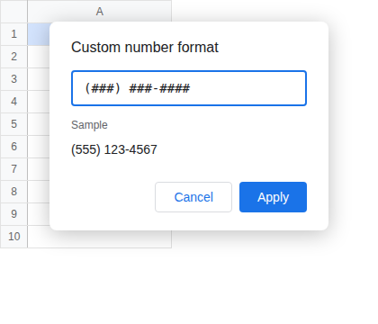
| You want | Custom format |
|---|---|
| (555) 123-4567 | (###) ###-#### |
| 555-123-4567 | ###-###-#### |
| +1 (555) 123-4567 | +1 (###) ###-#### |
| UK: +44 20 7946 0000 | "+44" ## #### #### |
2. Keep leading zeros and + signs
This is the #1 phone-number frustration. Because Sheets treats an entry like 07700900000 or +15551234567 as a number, it drops the leading zero and the plus. The fix is to store it as text instead:
- Format the column as plain text first — select it, then Format ▸ Number ▸ Plain text — before you type or paste. Everything stays exactly as entered, zeros and
+included. - Or prefix a single entry with an apostrophe: typing
'07700900000forces that cell to text and keeps the leading zero (the apostrophe itself doesn't show).
Numeric IDs (zips, codes) instead of phone numbers? If you need them to stay a real number but show a fixed number of digits, use 0 placeholders in a custom format — e.g. 00000 always shows five digits. For phone numbers, though, plain text is the safer choice because of the +.
3. "My format isn't working" — text vs numbers
If a custom number format seems to do nothing, your phone numbers are almost certainly stored as text (common after an import, or if they contain dashes, spaces, or parentheses). A number format only applies to values stored as numbers.
How to tell: by default, text is left-aligned and numbers are right-aligned. If your phone column is left-aligned, it's text.
To convert genuine digits from text to a number, wrap them in VALUE(); to go the other way (number → formatted text), use TEXT(). The next section combines both to clean things up in one step.
4. Clean up messy, inconsistent numbers
Real contact lists are rarely tidy — (555) 123 4567, 555.123.4567, and +1 555-123-4567 all mixed together. To standardize them, strip everything down to digits, then reformat.
Strip to digits only:
=REGEXREPLACE(A2, "\D", "")(\D matches any non-digit, so this removes spaces, dashes, dots, and parentheses.)
Strip and reformat to one consistent style in a single formula:
=TEXT(VALUE(REGEXREPLACE(A2, "\D", "")), "(000) 000-0000")That turns any of the messy versions above into (555) 123-4567. Using 0 placeholders (not #) guarantees all ten digits show.
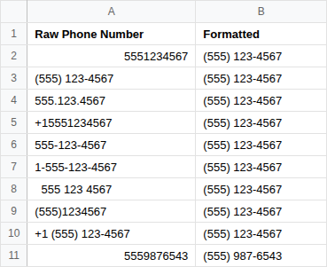
Or skip the formulas entirely. With Octo, connect your sheet and just say "clean and standardize the phone number column." It strips the mess and applies one consistent format across the whole column — no REGEXREPLACE required.
5. Format a whole column at once
For a display format, click the column header to select the entire column, then apply your custom number format — it covers every current cell and anything you add later.
For the standardizing formula, wrap it in ARRAYFORMULA so one formula fills the whole column:
=ARRAYFORMULA(IF(A2:A="", "", TEXT(VALUE(REGEXREPLACE(A2:A, "\D", "")), "(000) 000-0000")))6. Make numbers click-to-call
To turn a number into a clickable link (handy on shared or mobile sheets), use HYPERLINK with a tel: link:
=HYPERLINK("tel:" & A2, A2)Wrangling a messy contact list?
Octo connects to your Google Sheet and cleans, standardizes, and analyzes columns like these on command — in plain English, no formulas.
Add Octo to Chrome — freeFrequently asked questions
Why do my phone numbers lose the leading zero or + sign?
Sheets stores them as numbers and drops the leading zero and +. Format the cells as plain text (Format ▸ Number ▸ Plain text) before entering, or start the entry with an apostrophe (').
Why isn't my phone number format working?
A number format only applies to values stored as numbers. If your numbers are text (they'll be left-aligned), the format won't apply — convert them first.
How do I format a whole column at once?
Click the column header to select it, then Format ▸ Number ▸ Custom number format and enter your pattern; it applies to current and new entries.
How do I standardize inconsistent numbers?
Strip to digits with =REGEXREPLACE(A2,"\D",""), then reformat with =TEXT(VALUE(REGEXREPLACE(A2,"\D","")),"(000) 000-0000").
How do I make a phone number clickable?
Use =HYPERLINK("tel:"&A2, A2).
How we made this: We tested every format and formula in Google Sheets in 2026 to confirm the menu paths and results.